Descriptive Statistics
Contents
5. Descriptive Statistics
5.1. So Far…
We’ve gone over a lot of stuff so far and you all have been doing great with everything I’ve thrown at you
5.2. Measures of Descriptive Statistics
All descriptive statistics are either measures of central tendency or measures of variability, also known as measures of dispersion. Measures of central tendency focus on the average or middle values of data sets; whereas, measures of variability focus on the dispersion of data. These two measures use graphs, tables, and general discussions to help people understand the meaning of the analyzed data.
5.3. Central Tendency
Measures of central tendency describe the center position of a distribution for a data set. A person analyzes the frequency of each data point in the distribution and describes it using the mean, median, or mode, which measures the most common patterns of the analyzed data set.
from scipy import stats
import numpy as np
#make random data
nums=np.random.normal(0, 10, 1000)

import matplotlib.pyplot as plt

f, ax1 = plt.subplots()
ax1.hist(nums, bins='auto')
ax1.set_title('probability density (random)')
plt.tight_layout()
---------------------------------------------------------------------------
ModuleNotFoundError                       Traceback (most recent call last)
Input In [1], in <cell line: 1>()
----> 1 from scipy import stats
      2 import numpy as np
      3 #make random data

ModuleNotFoundError: No module named 'scipy'
f, ax1 = plt.subplots()
ax1.hist(nums, bins='auto')
ax1.set_title('probability density (random)')
plt.tight_layout()
ax1.plot([np.mean(nums)]*2,[0,100],'r')
#ax1.plot([np.median(nums)]*2,[0,100],'g')
# ax1.plot([stats.mode(nums)[0]]*2,[0,100],'g')
plt.show()

print("The Mean is: ",np.mean(nums))
print("The Mode is: ",stats.mode(nums))
print("The Median is: ",np.median(nums))
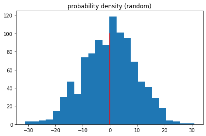
The Mean is:  -0.10101019622713875
The Mode is:  ModeResult(mode=array([-31.27902323]), count=array([1]))
The Median is:  0.32252726751052246
5.4. Dispersion
Measures of variability, or the measures of spread, aid in analyzing how spread-out the distribution is for a set of data. For example, while the measures of central tendency may give a person the average of a data set, it does not describe how the data is distributed within the set. So, while the average of the data may be 65 out of 100, there can still be data points at both 1 and 100. Measures of variability help communicate this by describing the shape and spread of the data set. Range, quartiles, absolute deviation, and variance are all examples of measures of variability. Consider the following data set: 5, 19, 24, 62, 91, 100. The range of that data set is 95, which is calculated by subtracting the lowest number (5) in the data set from the highest (100).
5.5. Range
The range is the simplest measure of variability to calculate, and one you have probably encountered many times in your life. The range is simply the highest score minus the lowest score
max_nums = max(nums)
min_nums = min(nums)
range_nums = max_nums-min_nums
print(max_nums)
print(min_nums)
print("The Range is :", range_nums)
30.927257895594554
-31.279023232798515
The Range is : 62.20628112839307
5.6. Standard deviation
The standard deviation is also a measure of the spread of your observations, but is a statement of how much your data deviates from a typical data point. That is to say, the standard deviation summarizes how much your data differs from the mean. This relationship to the mean is apparent in standard deviation’s calculation.

print(np.std(nums))
9.77196195814071
5.7. Variance
Often, standard deviation and variance are lumped together for good reason. The following is the equation for variance, does it look familiar?

Standard deviation looks at how spread out a group of numbers is from the mean, by looking at the square root of the variance. The variance measures the average degree to which each point differs from the mean—the average of all data points
print(np.var(nums))
95.49124051134919
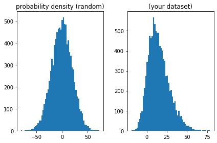
5.8. Shape
The skewness is a parameter to measure the symmetry of a data set and the kurtosis to measure how heavy its tails are compared to a normal distribution, see for example here.
import numpy as np
from scipy.stats import kurtosis, skew, skewnorm

n = 10000
start = 0
width = 20

a = 0
data_normal = skewnorm.rvs(size=n, a=a,loc = start, scale=width)

a = 3
data_skew = skewnorm.rvs(size=n, a=a,loc = start, scale=width)

import matplotlib.pyplot as plt

f, (ax1, ax2) = plt.subplots(1, 2)
ax1.hist(data_normal, bins='auto')
ax1.set_title('probability density (random)')
ax2.hist(data_skew, bins='auto')
ax2.set_title('(your dataset)')
plt.tight_layout()

sig1 = data_normal
print("mean : ", np.mean(sig1))
print("var  : ", np.var(sig1))
print("skew : ", skew(sig1))
print("kurt : ", kurtosis(sig1))
mean :  -0.220946743856605
var  :  396.1240367423572
skew :  -0.028057024589031802
kurt :  -0.022352653399519085
5.9. Correlation/Regression
5.9.1. Assumptions
The assumptions for Pearson correlation coefficient are as follows: level of measurement, related pairs, absence of outliers, normality of variables, linearity, and homoscedasticity.
Level of measurement refers to each variable. For a Pearson correlation, each variable should be continuous. If one or both of the variables are ordinal in measurement, then a Spearman correlation could be conducted instead.
Related pairs refers to the pairs of variables. Each participant or observation should have a pair of values. So if the correlation was between weight and height, then each observation used should have both a weight and a height value.
Absence of outliers refers to not having outliers in either variable. Having an outlier can skew the results of the correlation by pulling the line of best fit formed by the correlation too far in one direction or another. Typically, an outlier is defined as a value that is 3.29 standard deviations from the mean, or a standardized value of less than ±3.29.
Linearity and homoscedasticity refer to the shape of the values formed by the scatterplot. For linearity, a “straight line” relationship between the variable should be formed. If a line were to be drawn between all the dots going from left to right, the line should be straight and not curved. Homoscedasticity refers to the distance between the points to that straight line. The shape of the scatterplot should be tube-like in shape. If the shape is cone-like, then homoskedasticity would not be met.
import pandas as pd
path_to_data = '/Users/joe/Cook Share Dropbox/Joseph Nashed/NSCI Teaching/Lectures/Lectures1/Practice/rois.csv'
data_in = pd.read_csv(path_to_data).values
plt.scatter(data_in[:,1],data_in[:,2])
plt.xlabel('Height (inches)', size=18)
plt.ylabel('Weight (pounds)', size=18);
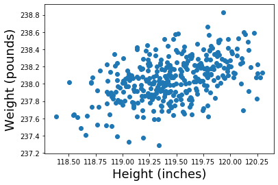
A scatter plot is a two dimensional data visualization that shows the relationship between two numerical variables — one plotted along the x-axis and the other plotted along the y-axis. Matplotlib is a Python 2D plotting library that contains a built-in function to create scatter plots the matplotlib.pyplot.scatter() function. ALWAYS PLOT YOUR RAW DATA
5.10. Pearson Correlation Coefficient
Correlation measures the extent to which two variables are related. The Pearson correlation coefficient is used to measure the strength and direction of the linear relationship between two variables. This coefficient is calculated by dividing the covariance of the variables by the product of their standard deviations and has a value between +1 and -1, where 1 is a perfect positive linear correlation, 0 is no linear correlation, and −1 is a perfect negative linear correlation. We can obtain the correlation coefficients of the variables of a dataframe by using the .corr() method. By default, Pearson correlation coefficient is calculated; however, other correlation coefficients can be computed such as, Kendall or Spearman
np.corrcoef(data_in[:,1],data_in[:,2])
array([[1.        , 0.45540708],
       [0.45540708, 1.        ]])
A rule of thumb for interpreting the size of the correlation coefficient is the following: 1–0.8 → Very strong 0.799–0.6 → Strong 0.599–0.4 → Moderate 0.399–0.2 → Weak 0.199–0 → Very Weak
5.11. Regression
Linear regression is an analysis that assesses whether one or more predictor variables explain the dependent (criterion) variable. The regression has five key assumptions:
Linear relationship Multivariate normality No or little multicollinearity No auto-correlation Homoscedasticity
A note about sample size. In Linear regression the sample size rule of thumb is that the regression analysis requires at least 20 cases per independent variable in the analysis.
import statsmodels.api as sm
X = data_in[:,1]
y = data_in[:,2]

# Note the difference in argument order
model = sm.OLS(y, X).fit()
predictions = model.predict(X) # make the predictions by the model

# Print out the statistics
model.summary()
---------------------------------------------------------------------------
ModuleNotFoundError                       Traceback (most recent call last)
<ipython-input-1-3c0f6fe3b2b1> in <module>()
----> 1 import statsmodels.api as sm
      2 X = data_in[:,1]
      3 y = data_in[:,2]
      4
      5 # Note the difference in argument order

ModuleNotFoundError: No module named 'statsmodels'
import pandas as pd
import numpy as np
import matplotlib.pyplot as plt
# import seaborn as seabornInstance
#from sklearn.model_selection import train_test_split
from sklearn.linear_model import LinearRegression
from sklearn import metrics

p1 = '/Users/joe/Cook Share Dropbox/Joseph Nashed/NSCI Teaching/Lectures/Lectures1/Practice/Weather.csv'
dataset = pd.read_csv(p1)
dataset.plot(x='MinTemp', y='MaxTemp', style='o')
plt.title('MinTemp vs MaxTemp')
plt.xlabel('MinTemp')
plt.ylabel('MaxTemp')
plt.show()
/Users/joe/anaconda3/envs/fmri/lib/python3.6/site-packages/IPython/core/interactiveshell.py:2785: DtypeWarning: Columns (7,8,18,25) have mixed types. Specify dtype option on import or set low_memory=False.
  interactivity=interactivity, compiler=compiler, result=result)
<Figure size 640x480 with 1 Axes>
X = dataset['MinTemp'].values.reshape(-1,1)
y = dataset['MaxTemp'].values.reshape(-1,1)
---------------------------------------------------------------------------
NameError                                 Traceback (most recent call last)
<ipython-input-58-1c0b57fd64d0> in <module>
----> 1 X = dataset['MinTemp'].values.reshape(-1,1)
      2 y = dataset['MaxTemp'].values.reshape(-1,1)

NameError: name 'dataset' is not defined
regressor = LinearRegression()
regressor.fit(X, y) #training the algorithm
y_pred = regressor.predict(X)
plt.scatter(X, y,  color='gray')
plt.plot(X, y_pred, color='red', linewidth=2)
plt.show()
---------------------------------------------------------------------------
NameError                                 Traceback (most recent call last)
<ipython-input-55-b8dea1654a62> in <module>
----> 1 regressor = LinearRegression()
      2 regressor.fit(X, y) #training the algorithm
      3 y_pred = regressor.predict(X)
      4 plt.scatter(X, y,  color='gray')
      5 plt.plot(X, y_pred, color='red', linewidth=2)

NameError: name 'LinearRegression' is not defined
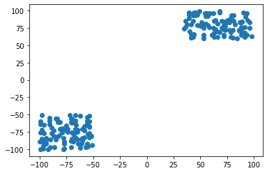
5.12. Another Example
import numpy as np
from sklearn.linear_model import LinearRegression
from sklearn import metrics
import matplotlib.pyplot as plt


x_vals1 = np.random.randint(-100,-50,100)
y_vals1 = np.random.randint(-100,-50,100)
x_vals2 = np.random.randint(35,100,100)
y_vals2 = np.random.randint(60,100,100)

x_t = np.concatenate((x_vals1,x_vals2))
y_t = np.concatenate((y_vals1,y_vals2))

plt.scatter(x_t, y_t)
plt.show()
regressor = LinearRegression().fit((x_t).reshape(-1,1),(y_t).reshape(-1,1))
y_pred = regressor.predict(x_t.reshape(-1,1))
plt.scatter(x_t, y_t)
plt.plot((x_t).reshape(-1,1), y_pred, color='red', linewidth=2)
plt.show()
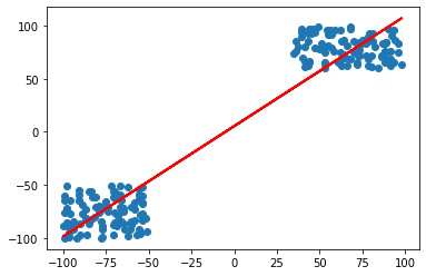
Whats wrong with this??
5.13. The Logic of Hypothesis Testing
State the Hypothesis: We state a hypothesis (guess) about a population. Usually the hypothesis concerns the value of a population parameter. … Gather Data: We obtain a random sample from the population. Make a Decision: We compare the sample data with the hypothesis about the population.
The Logic of Hypothesis Testing As just stated, the logic of hypothesis testing in statistics involves four steps. State the Hypothesis: We state a hypothesis (guess) about a population. Usually the hypothesis concerns the value of a population parameter. Define the Decision Method: We define a method to make a decision about the hypothesis. The method involves sample data. Gather Data: We obtain a random sample from the population. Make a Decision: We compare the sample data with the hypothesis about the population. Usually we compare the value of a statistic computed from the sample data with the hypothesized value of the population parameter. If the data are consistent with the hypothesis we conclude that the hypothesis is reasonable. NOTE: We do not conclude it is right, but reasonable! AND: We actually do this by rejecting the opposite hypothesis (called the NULL hypothesis). More on this later. If there is a big discrepency between the data and the hypothesis we conclude that the hypothesis was wrong. We expand on those steps in this section:
First Step: State the Hypothesis
Stating the hypothesis actually involves stating two opposing hypotheses about the value of a population parameter. Example: Suppose we have are interested in the effect of prenatal exposure of alcohol on the birth weight of rats. Also, suppose that we know that the mean birth weight of the population of untreated lab rats is 18 grams.
Here are the two opposing hypotheses:
The Null Hypothesis (Ho). This hypothesis states that the treatment has no effect. For our example, we formally state: The null hypothesis (Ho) is that prenatal exposure to alcohol has no effect on the birth weight for the population of lab rats. The birthweight will be equal to 18 grams. This is denoted
The Alternative Hypothesis (H1). This hypothesis states that the treatment does have an effect. For our example, we formally state: The alternative hypothesis (H1) is that prenatal exposure to alcohol has an effect on the birth weight for the population of lab rats. The birthweight will be different than 18 grams. This is denoted
Second Step: Define the Decision Method
We must define a method that lets us decide whether the sample mean is different from the hypothesized population mean. The method will let us conclude whether (reject null hypothesis) or not (accept null hypothesis) the treatment (prenatal alcohol) has an effect (on birth weight). We will go into details later.
Third Step: Gather Data.
Now we gather data. We do this by obtaining a random sample from the population. Example: A random sample of rats receives daily doses of alcohol during pregnancy. At birth, we measure the weight of the sample of newborn rats. The weights, in grams, are shown in the table.
We calculate the mean birth weight.
Experiment 1 Sample Mean = 13 Fourth Step: Make a Decision
We make a decision about whether the mean of the sample is consistent with our null hypothesis about the population mean. If the data are consistent with the null hypothesis we conclude that the null hypothesis is reasonable. Formally: we do not reject the null hypothesis.
If there is a big discrepency between the data and the null hypothesis we conclude that the null hypothesis was wrong. Formally: we reject the null hypothesis.
Example: We compare the observed mean birth weight with the hypothesized value, under the null hypothesis, of 18 grams.
If a sample of rat pups which were exposed to prenatal alcohol has a birth weight “near” 18 grams we conclude that the treatement does not have an effect. Formally: We do not reject the null hypothesis that prenatal exposure to alcohol has no effect on the birth weight for the population of lab rats.
If our sample of rat pups has a birth weight “far” from 18 grams we conclude that the treatement does have an effect. Formally: We reject the null hypothesis that prenatal exposure to alcohol has no effect on the birth weight for the population of lab rats.
For this example, we would probably decide that the observed mean birth weight of 13 grams is “different” than the value of 18 grams hypothesized under the null hypothesis. Formally: We reject the null hypothesis that prenatal exposure to alcohol has no effect on the birth weight for the population of lab rats.
5.14. Statistical significance
Statistical significance is the likelihood that a relationship between two or more variables is caused by something other than chance.
Statistical significance is used to provide evidence concerning the plausibility of the null hypothesis, which hypothesizes that there is nothing more than random chance at work in the data.
Statistical hypothesis testing is used to determine whether the result of a data set is statistically significant
Understanding Statistical Significance Statistical significance is a determination about the null hypothesis, which hypothesizes that the results are due to chance alone. A data set provides statistical significance when the p-value is sufficiently small.
When the p-value is large, then the results in the data are explainable by chance alone, and the data are deemed consistent with (while not proving) the null hypothesis.
When the p-value is sufficiently small (e.g., 5% or less), then the results are not easily explained by chance alone, and the data are deemed inconsistent with the null hypothesis; in this case the null hypothesis of chance alone as an explanation of the data is rejected in favor of a more systematic explanation
from scipy.stats import ttest_ind

for i in range(100):
    vals1 = np.random.rand(100)
    vals2 = np.random.rand(100)
    if ttest_ind(vals1,vals2)[1]<0.05:
        print(ttest_ind(vals1,vals2))
Ttest_indResult(statistic=-2.087309630290171, pvalue=0.03813997119746118)
Ttest_indResult(statistic=2.191484976341105, pvalue=0.029583341125764655)
Ttest_indResult(statistic=-2.3935353858603428, pvalue=0.017620578057267713)
5.15. Multiple Comparisons
Multiple comparisons arise when a statistical analysis involves multiple simultaneous statistical tests, each of which has a potential to produce a “discovery.” A stated confidence level generally applies only to each test considered individually, but often it is desirable to have a confidence level for the whole family of simultaneous tests. Failure to compensate for multiple comparisons can have important real-world consequences, as illustrated by the following examples:
Suppose the treatment is a new way of teaching writing to students, and the control is the standard way of teaching writing. Students in the two groups can be compared in terms of grammar, spelling, organization, content, and so on. As more attributes are compared, it becomes increasingly likely that the treatment and control groups will appear to differ on at least one attribute due to random sampling error alone. Suppose we consider the efficacy of a drug in terms of the reduction of any one of a number of disease symptoms. As more symptoms are considered, it becomes increasingly likely that the drug will appear to be an improvement over existing drugs in terms of at least one symptom.
5.16. Different Test Statistics
A test statistic is a random variable that is calculated from sample data and used in a hypothesis test. You can use test statistics to determine whether to reject the null hypothesis. The test statistic compares your data with what is expected under the null hypothesis.
A test statistic measures the degree of agreement between a sample of data and the null hypothesis. Its observed value changes randomly from one random sample to a different sample. A test statistic contains information about the data that is relevant for deciding whether to reject the null hypothesis. The sampling distribution of the test statistic under the null hypothesis is called the null distribution. When the data show strong evidence against the assumptions in the null hypothesis, the magnitude of the test statistic becomes too large or too small depending on the alternative hypothesis. This causes the test’s p-value to become small enough to reject the null hypothesis.
Different hypothesis tests make different assumptions about the distribution of the random variable being sampled in the data. These assumptions must be considered when choosing a test and when interpreting the results.
5.17. Z-Stat
The z-test assumes that the data are independently sampled from a normal distribution. Secondly, it assumes that the standard deviation σ of the underlying normal distribution is known;
5.18. t-Stat
The t-test also assumes that the data are independently sampled from a normal distribution. but unlike the F-Test it assumes it does not make assumptions about the standard deviation σ of the underlying normal distribution
5.19. F-Stat
An F-test assumes that data are normally distributed and that samples are independent from one another. Data that differs from the normal distribution could be due to a few reasons. The data could be skewed or the sample size could be too small to reach a normal distribution. Regardless the reason, F-tests assume a normal distribution and will result in inaccurate results if the data differs significantly from this distribution.
F-tests also assume that data points are independent from one another. For example, you are studying a population of giraffes and you want to know how body size and sex are related. You find that females are larger than males, but you didn’t take into consideration that substantially more of the adults in the population are female than male. Thus, in your dataset, sex is not independent from age.